Working with many packages

set.seed(1234)

In practice, most R analyses load a handful of packages at once. That’s great — each package solves a specific problem — but it also creates two challenges:

Conflicts: two packages may export a function with the same name.
Compatibility: does the output of one package feed naturally into the next?

This lesson covers both.

Some data to work on

library(tibble)

n <- 500
df <- tibble(
  id      = 1:n,
  age     = rnorm(n, mean = 55, sd = 12) |> round(),
  sex     = sample(c("Male", "Female"), n, replace = TRUE),
  smoker  = sample(c(TRUE, FALSE), n, replace = TRUE, prob = c(0.3, 0.7)),
  sbp     = round(120 + 0.4 * age + 8 * smoker + rnorm(n, sd = 12)),
  bmi     = round(rnorm(n, mean = 26, sd = 4), 1)
)

df |> head(8) |> gt::gt(id = "patient_tbl")

id	age	sex	smoker	sbp	bmi
1	41	Female	FALSE	122	33.2
2	58	Male	FALSE	147	20.5
3	68	Female	FALSE	129	23.2
4	27	Male	TRUE	146	23.8
5	60	Female	TRUE	160	24.8
6	61	Female	TRUE	130	24.5
7	48	Male	FALSE	150	27.8
8	48	Male	TRUE	145	21.0

Loading order and function masking

Every time you call library(pkg), R attaches the package to the search path — a list of environments R looks through, left to right, when you type a name.

search()

 [1] ".GlobalEnv"        "package:tibble"    "package:stats"    
 [4] "package:graphics"  "package:grDevices" "package:utils"    
 [7] "package:datasets"  "package:methods"   "Autoloads"        
[10] "package:base"

The last package you load sits at position 2 (just after .GlobalEnv), so its functions are found first. When two packages share a function name, the one loaded later silently masks the earlier one.

A concrete example

Both {dplyr} and {MASS} have a function called select(). After library(MASS), typing select() calls the MASS version — the dplyr one is still there, just hidden.

library(dplyr)


Attaching package: 'dplyr'

The following objects are masked from 'package:stats':

    filter, lag

The following objects are masked from 'package:base':

    intersect, setdiff, setequal, union

library(MASS)


Attaching package: 'MASS'

The following object is masked from 'package:dplyr':

    select

R warns you but proceeds - there’s no guarantee you will notice the warning message in a busy session. But once you try to use it, you may see the function isn’t working:

df |> select(id, age, sbp) |> head(3)

Error in `select()`:
! unused arguments (id, age, sbp)

In the case of select() here, you find out eventually. However, in some cases you might not notice the problem, because the function runs but just outputs something other than what you intended. These are the real errors that can cause silent bugs in your code.

Three solutions to masking

1. Explicit namespacing with `::`

A safe but potentially arduous habit: write pkg::function() for any function that might be ambiguous.

df |> dplyr::select(id, age, sbp) |> head(3)

# A tibble: 3 × 3
     id   age   sbp
  <int> <dbl> <dbl>
1     1    41   122
2     2    58   147
3     3    68   129

This works even when a function is masked, and makes code easier to read and share.

2. The `{conflicted}` package

{conflicted} turns silent masking into a loud error, forcing you to be explicit. Load it at the top of your script and every ambiguous call will stop with a helpful message.

library(conflicted)

df |> filter(age > 70) |> head(5)

Error:
! [conflicted] filter found in 2 packages.
Either pick the one you want with `::`:
• dplyr::filter
• stats::filter
Or declare a preference with `conflicts_prefer()`:
• `conflicts_prefer(dplyr::filter)`
• `conflicts_prefer(stats::filter)`

You resolve the conflict once using conflict_prefer(name, winner, losers = NULL):

conflict_prefer("filter", "dplyr")

[conflicted] Will prefer dplyr::filter over any other package.

Now filter() unambiguously refers to the dplyr version for the rest of the session.

df |> filter(age > 70) |> head(5)

# A tibble: 5 × 6
     id   age sex    smoker   sbp   bmi
  <int> <dbl> <chr>  <lgl>  <dbl> <dbl>
1    20    84 Male   FALSE    139  18.4
2    41    72 Male   TRUE     159  23.5
3    57    75 Female FALSE    147  15.8
4    59    74 Male   FALSE    151  30.9
5    62    86 Male   FALSE    151  21.6

3. `{box}`: surgical package imports

An alternative to library() is the {box} package. Instead of loading an entire package namespace, you import only the specific functions you need.

box::use(
  dplyr[filter, select, mutate],   # only these three functions from dplyr
  ggplot2[ggplot, aes, geom_point], # only these from ggplot2
  MASS[mass_select = select] # rename MASS::select to mass_select to avoid conflict with dplyr
)

This is especially useful in packages, larger codebases, or when you want the code to be completely explicit about where every function comes from.

Tip

For day-to-day scripts, library() with explicit namespacing (pkg::function()) + {conflicted} is usually enough.

{box} becomes attractive in package development or when you want strict, reproducible namespacing.

Cross-package workflows

A lot of R’s power comes from packages that are designed to talk to each other. The key idea: if a function always returns a standard, predictable object (like a data frame or a specific class), other packages can be written to work with it directly.

Generic functions and methods

Base R uses generics — functions like summary(), print(), and predict() — that behave differently depending on what they are given.

Let’s set up a linear model:

m <- lm(sbp ~ age + sex + smoker + bmi, data = df)
class(m)

[1] "lm"

The native print output:


Call:
lm(formula = sbp ~ age + sex + smoker + bmi, data = df)

Coefficients:
(Intercept)          age      sexMale   smokerTRUE          bmi  
  116.77237      0.47330      0.04204      8.85407     -0.02542

summary() recognises it as a linear model and formats accordingly:

summary(m)


Call:
lm(formula = sbp ~ age + sex + smoker + bmi, data = df)

Residuals:
    Min      1Q  Median      3Q     Max 
-36.063  -7.379   0.471   7.810  32.268 

Coefficients:
             Estimate Std. Error t value Pr(>|t|)    
(Intercept) 116.77237    4.00266  29.174  < 2e-16 ***
age           0.47330    0.04061  11.655  < 2e-16 ***
sexMale       0.04204    1.01365   0.041    0.967    
smokerTRUE    8.85407    1.13957   7.770 4.58e-14 ***
bmi          -0.02542    0.12324  -0.206    0.837    
---
Signif. codes:  0 '***' 0.001 '**' 0.01 '*' 0.05 '.' 0.1 ' ' 1

Residual standard error: 11.26 on 495 degrees of freedom
Multiple R-squared:  0.2907,    Adjusted R-squared:  0.285 
F-statistic: 50.72 on 4 and 495 DF,  p-value: < 2.2e-16

This system — called S3 dispatch — means that different packages can teach the same verb new tricks, without you having to learn a different function name.

Under the hood, R looks at the class of the object you pass to summary(), sees it’s a lm object, and calls the specialised summary.lm() automatically.

Standardised outputs: the tidy principle

The tidyverse is built on a simple idea: data in, data out. Each function takes a data frame and returns a data frame, making operations easy to chain.

Many packages outside the core tidyverse follow the same principle. The key package here is {broom}, which converts messy model objects into tidy tibbles.

library(broom)

broom::tidy() extracts the coefficients as a clean tibble:

broom::tidy(m, conf.int = TRUE)

# A tibble: 5 × 7
  term        estimate std.error statistic   p.value conf.low conf.high
  <chr>          <dbl>     <dbl>     <dbl>     <dbl>    <dbl>     <dbl>
1 (Intercept) 117.        4.00     29.2    1.32e-109  109.      125.   
2 age           0.473     0.0406   11.7    6.58e- 28    0.394     0.553
3 sexMale       0.0420    1.01      0.0415 9.67e-  1   -1.95      2.03 
4 smokerTRUE    8.85      1.14      7.77   4.58e- 14    6.62     11.1  
5 bmi          -0.0254    0.123    -0.206  8.37e-  1   -0.268     0.217

broom::glance() gives one-row model-level summaries:

broom::glance(m)

# A tibble: 1 × 12
  r.squared adj.r.squared sigma statistic  p.value    df logLik   AIC   BIC
      <dbl>         <dbl> <dbl>     <dbl>    <dbl> <dbl>  <dbl> <dbl> <dbl>
1     0.291         0.285  11.3      50.7 8.77e-36     4 -1918. 3847. 3873.
# ℹ 3 more variables: deviance <dbl>, df.residual <int>, nobs <int>

broom::augment() adds fitted values and residuals back to your data:

broom::augment(m, df) |> 
  dplyr::select(id, sbp, .fitted, .resid) |> 
  head(5)

# A tibble: 5 × 4
     id   sbp .fitted .resid
  <int> <dbl>   <dbl>  <dbl>
1     1   122    135. -13.3 
2     2   147    144.   3.26
3     3   129    148. -19.4 
4     4   146    138.   8.16
5     5   160    153.   6.61

Because tidy() always returns a tibble with the same column names (term, estimate, std.error, p.value, …), the output easily plugs into {ggplot2}:

library(ggplot2)

broom::tidy(m, conf.int = TRUE) |>
  filter(term != "(Intercept)") |>
  ggplot(aes(x = estimate, xmin = conf.low, xmax = conf.high, y = term)) +
  geom_pointrange()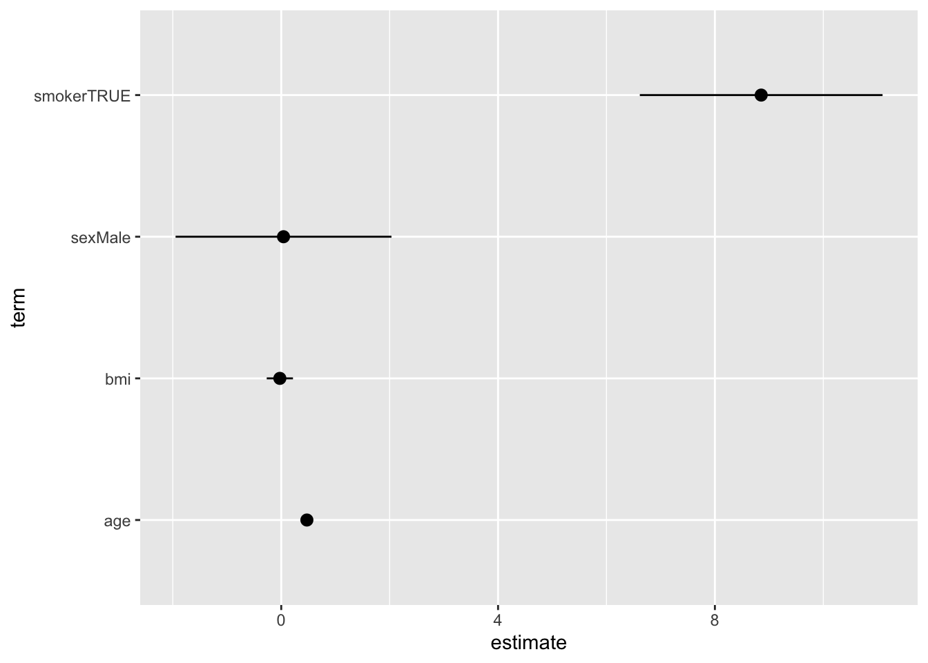

`{gtsummary}`: a complete cross-package workflow

{gtsummary} is a good example of a package that slots into a tidy workflow seamlessly. It takes standard R model objects and produces publication-ready tables, using the same underlying ideas. Here, using tbl_regression():

library(gtsummary)

m |>
  tbl_regression(
    label = list(
      age    ~ "Age (years)",
      sex    ~ "Sex",
      smoker ~ "Smoker",
      bmi    ~ "BMI (kg/m²)"
    )
  ) |>
  bold_p() |>
  bold_labels()

Characteristic	Beta	95% CI	p-value
Age (years)	0.47	0.39, 0.55	<0.001
Sex
Female	—	—
Male	0.04	-1.9, 2.0	>0.9
Smoker
FALSE	—	—
TRUE	8.9	6.6, 11	<0.001
BMI (kg/m²)	-0.03	-0.27, 0.22	0.8
Abbreviation: CI = Confidence Interval

No need to manually extract and format coefficients — {gtsummary} calls broom::tidy() internally, giving you a formatted table in two lines.

Note

{gtsummary} works with a wide range of model types: lm, glm, coxph (survival), lme4 mixed models, and more — all using the same tbl_regression() call.

Another example: survival analysis

The same pattern works with survival models from the {survival} package:

library(survival)

# Simulate a time-to-event outcome:
df2 <- df |> mutate(
  time  = rexp(n, rate = 0.05),
  event = rbinom(n, 1, prob = 0.6)
)

cox_m <- coxph(Surv(time, event) ~ age + sex + smoker, data = df2)

{broom} and {gtsummary} work exactly the same way:

cox_m |> broom::tidy(exponentiate = TRUE, conf.int = TRUE)

# A tibble: 3 × 7
  term       estimate std.error statistic p.value conf.low conf.high
  <chr>         <dbl>     <dbl>     <dbl>   <dbl>    <dbl>     <dbl>
1 age           1.01    0.00485     1.36    0.173    0.997      1.02
2 sexMale       1.21    0.120       1.57    0.116    0.955      1.53
3 smokerTRUE    0.874   0.137      -0.978   0.328    0.668      1.14

cox_m |>
  tbl_regression(
    exponentiate = TRUE)

Characteristic	HR	95% CI	p-value
age	1.01	1.00, 1.02	0.2
sex
Female	—	—
Male	1.21	0.95, 1.53	0.12
smoker
FALSE	—	—
TRUE	0.87	0.67, 1.14	0.3
Abbreviations: CI = Confidence Interval, HR = Hazard Ratio

A more general principle: design for interoperability

The tidy principle

Functions that take and return data frames with predictable structure — is a powerful design pattern that encourages interoperability between packages.

When you choose packages for your workflow, look for ones that follow this principle.

Understanding function inputs and outputs

When you use a new package, take time to understand what its functions expect as input and what they return.

Start with ?pkg::fn to read the documentation and go to the package website / vignettes (= user manuals). Then experiment with simple examples to see the output structure.

Once you know the input requirements and the output format, try playing with the output yourself. Take you time to manually inspect and manipulate the output into different formats; e.g., tables, plots, etc.

Once you understand this, it’s time to see how you can use the output in your workflow, and which other packages fit well into the workflow.

Key takeaways

Problem	Solution
Silent function masking	Use `pkg::fn()` or load `{conflicted}`
Want to resolve a conflict once	`conflict_prefer("fn", "pkg")`
Want zero namespace pollution	`box::use(pkg[fn1, fn2])`
Understand your function inputs/outputs	`?pkg::fn`
Model output hard to work with	`broom::tidy()` / `broom::glance()`
Need a publication table fast	`gtsummary::tbl_regression()`

Some data to work on

Loading order and function masking

A concrete example

Three solutions to masking

1. Explicit namespacing with ::

2. The {conflicted} package

3. {box}: surgical package imports

Cross-package workflows

Generic functions and methods

Standardised outputs: the tidy principle

{gtsummary}: a complete cross-package workflow

Another example: survival analysis

A more general principle: design for interoperability

The tidy principle

Understanding function inputs and outputs

Key takeaways

Further reading

1. Explicit namespacing with `::`

2. The `{conflicted}` package

3. `{box}`: surgical package imports

`{gtsummary}`: a complete cross-package workflow