library(tidyverse)
set.seed(1234)More Tidyverse
The tidyverse is a collection of packages built for a common style of data analysis. The idea is simple: keep data in tidy columns, then solve tasks by chaining clear verbs.
Some data to work on
n <- 1000
df <- tibble(
  id = 1:n,
  date = sample(
    seq(ymd("2024-01-01"), ymd("2024-12-31"), by = "days"),
    n, replace = TRUE
  ),
  age = rnorm(n, mean = 40, sd = 10) |> round(),
  sex = sample(
    c("M", "F"),
    n, replace = TRUE
  ),
  weight = rnorm(n, mean = 75, sd = 10) |> round(),
  height = (rnorm(n, mean = 163, sd = 7) + (date - ymd("2024-01-01")) / 36.5 + (sex == "M")*7) |> as.numeric() |> round(),
  note = sample(
    c("new-patient", "follow-up", "urgent"),
    n, replace = TRUE
  ) |> factor()
)

df |> head(10) |> gt::gt(id = "patients_tbl")| id | date | age | sex | weight | height | note |
|---|---|---|---|---|---|---|
| 1 | 2024-10-10 | 49 | F | 59 | 174 | new-patient |
| 2 | 2024-12-01 | 43 | M | 87 | 175 | urgent |
| 3 | 2024-04-10 | 41 | M | 68 | 174 | new-patient |
| 4 | 2024-04-20 | 34 | F | 84 | 167 | new-patient |
| 5 | 2024-05-12 | 42 | F | 74 | 170 | follow-up |
| 6 | 2024-04-07 | 38 | F | 76 | 164 | urgent |
| 7 | 2024-04-12 | 41 | M | 80 | 174 | urgent |
| 8 | 2024-08-01 | 34 | M | 66 | 170 | urgent |
| 9 | 2024-03-30 | 52 | F | 74 | 159 | follow-up |
| 10 | 2024-11-21 | 51 | M | 68 | 177 | new-patient |
dplyr in one minute
{dplyr} is for data manipulation with readable verbs. Most common pattern: data |> filter(...) |> mutate(...) |> summarise(...).
tidyr: reshape data
{tidyr} helps move between wide and long data and fill missing values.
pivot_longer() and pivot_wider()
These are ways of reshaping data. Let’s start with a dataset in wide format:
mortality_df <- tibble(
  group = c("A", "B"),
  mort_6mo = c(0.1,0.15),
  mort_1yr = c(0.2,0.25),
  mort_2yr = c(0.3,0.35),
  mort_5yr = c(0.5,0.55)
)
mortality_df |> gt::gt()| group | mort_6mo | mort_1yr | mort_2yr | mort_5yr |
|---|---|---|---|---|
| A | 0.10 | 0.20 | 0.30 | 0.50 |
| B | 0.15 | 0.25 | 0.35 | 0.55 |
Now let’s make it long:
mortality_df_long <- mortality_df |> pivot_longer(
  cols = c(mort_6mo, mort_1yr, mort_2yr, mort_5yr),
  names_to = "time",
  values_to = "mortality",
  names_pattern = "mort_(.*)"
)

mortality_df_long |> gt::gt()| group | time | mortality |
|---|---|---|
| A | 6mo | 0.10 |
| A | 1yr | 0.20 |
| A | 2yr | 0.30 |
| A | 5yr | 0.50 |
| B | 6mo | 0.15 |
| B | 1yr | 0.25 |
| B | 2yr | 0.35 |
| B | 5yr | 0.55 |
To go the other way, we can widen it back (notice, we have control over how column names are transformed into row values, and vice versa):
mortality_df_long |> pivot_wider(
  names_from = time,
  names_glue = "{time}_{.value}",
  values_from = mortality
) |> gt::gt()| group | 6mo_mortality | 1yr_mortality | 2yr_mortality | 5yr_mortality |
|---|---|---|---|---|
| A | 0.10 | 0.20 | 0.30 | 0.50 |
| B | 0.15 | 0.25 | 0.35 | 0.55 |
separate_wider_delim()
A simple way of splitting a column into multiple columns based on a delimiter:
data.frame(
  x = c("A_1", "B_2", "C_1", "D_2", "E_2")
) |> gt::gt()| x |
|---|
| A_1 |
| B_2 |
| C_1 |
| D_2 |
| E_2 |
data.frame(
  x = c("A_1", "B_2", "C_1", "D_2", "E_2")
) |> separate_wider_delim(
  x, delim = "_",
  names = c("letter", "number")
) |> gt::gt()| letter | number |
|---|---|
| A | 1 |
| B | 2 |
| C | 1 |
| D | 2 |
| E | 2 |
Other tidyverse packages (quick tour)
readr (import text data)
Purpose: fast, friendly file import. Useful functions: read_csv(), read_tsv(), write_csv().
Tip
Other nice packages are {readxl} for Excel files and {googlesheets4} for Google Sheets along with {tidyxl} for non-tabular Excel files.
tibble (modern data frame)
Tibbles are a special type of data.frame, providing a few benefits; cleaner printing and safer column handling. In addition, building tibbles allow you to build the columns sequentially (i.e., you can refer to columns created earlier in the same tibble() call).
tibble(
  x = 1:3,
  y = x*3
) |> gt::gt()| x | y |
|---|---|
| 1 | 3 |
| 2 | 6 |
| 3 | 9 |
Also comes with add_row():
df |>
  head(5) |>
  add_row(id = -1, date = ymd("2024-05-05"), sex = "M") |>
gt::gt()| id | date | age | sex | weight | height | note |
|---|---|---|---|---|---|---|
| 1 | 2024-10-10 | 49 | F | 59 | 174 | new-patient |
| 2 | 2024-12-01 | 43 | M | 87 | 175 | urgent |
| 3 | 2024-04-10 | 41 | M | 68 | 174 | new-patient |
| 4 | 2024-04-20 | 34 | F | 84 | 167 | new-patient |
| 5 | 2024-05-12 | 42 | F | 74 | 170 | follow-up |
| -1 | 2024-05-05 | NA | M | NA | NA | NA |
purrr (iterate without explicit loops)
A clean way of applying functions to subsets (see previous lesson on Loops and parallelisation). Useful functions: map(), map_dbl(), map2().
df |>
  select(weight, sex) |>
  group_by(sex) |>
  summarise(mean_weight = mean(weight)) |>
gt::gt()| sex | mean_weight |
|---|---|
| F | 74.91634 |
| M | 75.69136 |
split(df$weight, df$sex) |>
purrr::map_dfr(mean) |> gt::gt()| F | M |
|---|---|
| 74.91634 | 75.69136 |
stringr (string handling)
Purpose: consistent string tools. Useful functions: str_detect(), str_replace(), str_extract().
c("word", "hypenated-word", "unhyphenated word") |> str_detect("-")[1] FALSE TRUE FALSEdf |> head(5) |> gt::gt()| id | date | age | sex | weight | height | note |
|---|---|---|---|---|---|---|
| 1 | 2024-10-10 | 49 | F | 59 | 174 | new-patient |
| 2 | 2024-12-01 | 43 | M | 87 | 175 | urgent |
| 3 | 2024-04-10 | 41 | M | 68 | 174 | new-patient |
| 4 | 2024-04-20 | 34 | F | 84 | 167 | new-patient |
| 5 | 2024-05-12 | 42 | F | 74 | 170 | follow-up |
df |>
  filter(
    str_detect(note, "-")
  ) |>
  mutate(
    note_clean = str_replace(note, "-", " ")
  ) |>
head(5) |> gt::gt()| id | date | age | sex | weight | height | note | note_clean |
|---|---|---|---|---|---|---|---|
| 1 | 2024-10-10 | 49 | F | 59 | 174 | new-patient | new patient |
| 3 | 2024-04-10 | 41 | M | 68 | 174 | new-patient | new patient |
| 4 | 2024-04-20 | 34 | F | 84 | 167 | new-patient | new patient |
| 5 | 2024-05-12 | 42 | F | 74 | 170 | follow-up | follow up |
| 9 | 2024-03-30 | 52 | F | 74 | 159 | follow-up | follow up |
forcats (factor handling)
Purpose: robust factor workflows. Useful functions: fct_relevel(), fct_reorder(), fct_lump().
df$note |> levels()[1] "follow-up" "new-patient" "urgent" z <- df |> mutate(
note = fct_relevel(note, "follow-up", after = 3)
)
z$note |> levels()[1] "new-patient" "urgent" "follow-up" lubridate (dates and times)
Purpose: parse and manipulate dates. Useful functions: ymd(), wday(), floor_date().
df |>
  select(id, date) |>
  mutate(
    weekday = wday(date, label = T),
    prior_monday = floor_date(date, "week", week_start = 1)
  ) |>
head(5) |> gt::gt()| id | date | weekday | prior_monday |
|---|---|---|---|
| 1 | 2024-10-10 | Thu | 2024-10-07 |
| 2 | 2024-12-01 | Sun | 2024-11-25 |
| 3 | 2024-04-10 | Wed | 2024-04-08 |
| 4 | 2024-04-20 | Sat | 2024-04-15 |
| 5 | 2024-05-12 | Sun | 2024-05-06 |
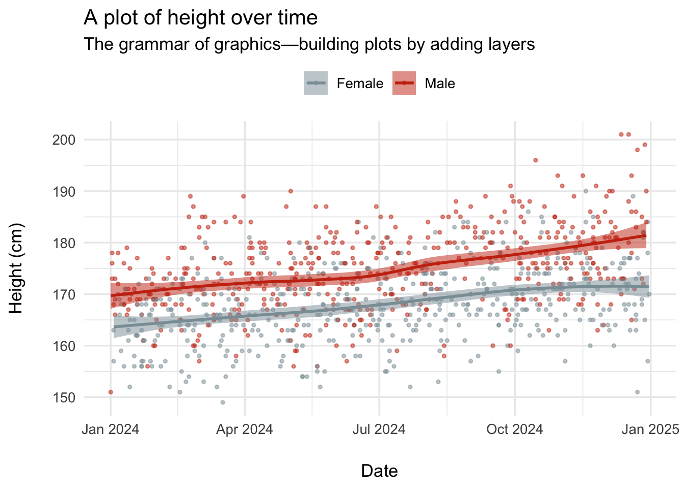
ggplot2: a future lesson topic
library(wesanderson)
df |>
  ggplot(aes(x = date, y = height, color = sex, fill = sex)) +
  geom_point(size = 1.5, alpha = 0.5, shape =20) +
  geom_smooth(method = "loess", formula = y~x, linewidth = 1, alpha = 0.5) +
  labs(
    title = "A plot of height over time",
    subtitle = "The grammar of graphics—building plots by adding layers",
    x = "Date",
    y = "Height (cm)",
    color = NULL
  ) +
  theme_minimal(base_size = 13) +
  theme(
    legend.position = "top",
    axis.title.x = element_text(margin = margin(t = 20)),
    axis.title.y = element_text(margin = margin(r = 20))
  ) +
  scale_color_manual(values = wes_palette("Royal1"), labels = c("F" = "Female", "M" = "Male")) +
  scale_fill_manual(values = wes_palette("Royal1"), labels = c("F" = "Female", "M" = "Male"), name=NULL)