Data types and structures

library(dplyr)
library(ggplot2)

Terminology: Objects and classes

Objects & variables

Everything in your environment has a name (variable) and a value (object)

Classes

Specific sets of attributes that define different types of objects

Basic data types

Numerics

Integers

x <- 1L

typeof(1:5)

[1] "integer"

class(1L)

[1] "integer"

Doubles

x <- 1.3

typeof(x)

[1] "double"

class(x)

[1] "numeric"

However, both can be seen as instances of numeric:

is.numeric(1L)

[1] TRUE

is.numeric(1.3)

[1] TRUE

Complex

6i

[1] 0+6i

typeof(6i)

[1] "complex"

Character

"Hello"

[1] "Hello"

typeof("Hello")

[1] "character"

Logical

TRUE

[1] TRUE

FALSE

[1] FALSE

NA

[1] NA

typeof(c(T,F,NA))

[1] "logical"

Raw

"Hello" |> charToRaw()

[1] 48 65 6c 6c 6f

"Hello" |> charToRaw() |> rawToBits()

 [1] 00 00 00 01 00 00 01 00 01 00 01 00 00 01 01 00 00 00 01 01 00 01 01 00 00
[26] 00 01 01 00 01 01 00 01 01 01 01 00 01 01 00

8 |> intToBits()

 [1] 00 00 00 01 00 00 00 00 00 00 00 00 00 00 00 00 00 00 00 00 00 00 00 00 00
[26] 00 00 00 00 00 00 00

Vectors

Numeric vector:

c(1,3,4,2)

[1] 1 3 4 2

Character vector:

c("Word1", "Word2", "Word3")

[1] "Word1" "Word2" "Word3"

Logical vector:

c(TRUE, FALSE, TRUE, NA)

[1]  TRUE FALSE  TRUE    NA

Empty vector:

c(TRUE, FALSE)[0]

logical(0)

c("hello", "world")[0]

character(0)

c(1.0, 2.3)[0]

numeric(0)

c(1L, 4L)[0]

integer(0)

Actually, it was all vectors all along:

c(1) == 1

[1] TRUE

Type coercion

Every element in a vector must have the same type

c(1, "Hello")

[1] "1"     "Hello"

# Notice, the num 1 is coerced into "1" (a character)

Combining vectors

vec1 <- 1:3
vec2 <- 5

c(vec1, vec2)

[1] 1 2 3 5

c(vec1, 4, 5)

[1] 1 2 3 4 5

Larger structures

Matrices - vectors in higher dimensions

matrix(1:6, nrow = 3, ncol = 2)

     [,1] [,2]
[1,]    1    4
[2,]    2    5
[3,]    3    6

Type coercion

c("Hello", 1:4) |> matrix(nrow = 3, ncol = 2)

Warning in matrix(c("Hello", 1:4), nrow = 3, ncol = 2): data length [5] is not
a sub-multiple or multiple of the number of rows [3]

     [,1]    [,2]   
[1,] "Hello" "3"    
[2,] "1"     "4"    
[3,] "2"     "Hello"

Creating a matrix by changing dimensionality of a vector

m <- c(1:18)
m

 [1]  1  2  3  4  5  6  7  8  9 10 11 12 13 14 15 16 17 18

dim(m) <- c(3,3,2)
m

, , 1

     [,1] [,2] [,3]
[1,]    1    4    7
[2,]    2    5    8
[3,]    3    6    9

, , 2

     [,1] [,2] [,3]
[1,]   10   13   16
[2,]   11   14   17
[3,]   12   15   18

Lists

Lists can contain elements of different class/type and length, and elements can be named:

list1 <- list(
  a = c("a", "b"),
  b = c(TRUE, FALSE, TRUE, TRUE),
  "Some text here",
  c = NULL,
  "More text"
)
list1

$a
[1] "a" "b"

$b
[1]  TRUE FALSE  TRUE  TRUE

[[3]]
[1] "Some text here"

$c
NULL

[[5]]
[1] "More text"

(Actually, vectors can also have named elements)

Data.frames

df <- data.frame(
  x = 1:4, 
  y = c(100,200,100,200),
  z = c("word1", "word2", "word3", "word4")
)
df

  x   y     z
1 1 100 word1
2 2 200 word2
3 3 100 word3
4 4 200 word4

list2 <- list(
  a = c("a", "b"),
  b = c(TRUE, FALSE, TRUE, TRUE),
  c = NULL,
  df,
  my_plot = df |> ggplot(aes(x=x, y=y)) + geom_point()
)
list2

$a
[1] "a" "b"

$b
[1]  TRUE FALSE  TRUE  TRUE

$c
NULL

[[4]]
  x   y     z
1 1 100 word1
2 2 200 word2
3 3 100 word3
4 4 200 word4

$my_plot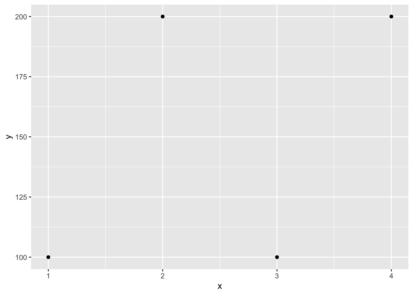

Other types and structures

Factors

Character vectors with specific levels

c("cat", "c", "Dog", "Dog", "cat") |> 
  factor(levels = c("cat", "c", "Dog"), 
         labels = c("Cat", "Cat", "Dog"))

[1] Cat Cat Dog Dog Cat
Levels: Cat Dog

Dates and Date-times (yyyy-mm-dd)

# Types
"1970-01-01" |> as.Date()

[1] "1970-01-01"

"2001-04-01 07:30:00" |> as.POSIXct()

[1] "2001-04-01 07:30:00 CEST"

Notes, dates start at 1970-01-01

# Day 0
as.Date(0)

[1] "1970-01-01"

as.numeric(as.Date("1969-01-01"))

[1] -365

Because dates are just numbers behind-the-scenes, R can directly plot dates

# Plotting and calculations
df_n <- 500
df <- tibble::tibble(
  date = as.Date(runif(df_n, min = 0, max = 730)),
  y = as.numeric(date) * 0.2 + rnorm(df_n, 0, 100)
)

with(df, plot(date, y, pch="."))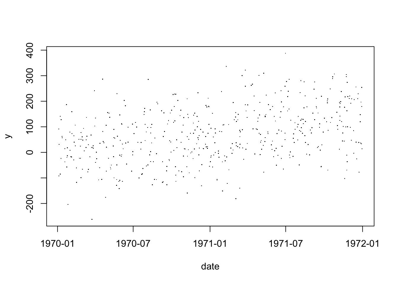

And even perform regression analyses on them

df |> ggplot(aes(x = date, y = y)) +
  geom_point(alpha = 0.2, size = .6) +
  geom_smooth(method = "lm", formula = y~x, se = T)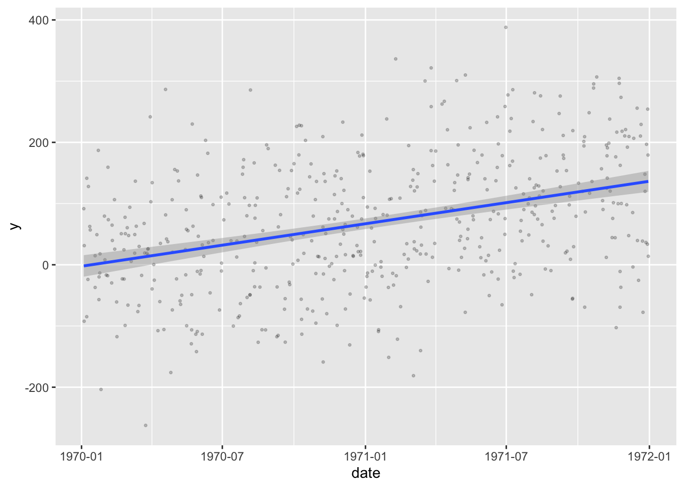

Difftime objects

diff <- as.Date("1970-01-01") - as.Date("1960-01-01")
diff

Time difference of 3653 days

Tibble (tidyverse)

Tibbles are built sequentially (i.e., each column is created before the next one); this means that the values from one column can be used in defining the values of the next

tibble <- tibble(x=1:5, 
                 y = x + 5)

Subsetting a single column from a tibble allows you to keep the data in tibble-form, whereas subsetting a single column from a df usually gives just the vector that formed that column

df <- data.frame(x=1:5, 
                 y = 6:10)
df[,"y"]

[1]  6  7  8  9 10

tibble[,"y"]

# A tibble: 5 × 1
      y
  <dbl>
1     6
2     7
3     8
4     9
5    10

# Unless you use the $ operator
tibble$y

[1]  6  7  8  9 10

Data.table

A layer on top of data.frames. Comes from the {data.table} package. Useful for writing concise code and lightning fast for very large datasets.

Regular expressions

These are pattern matching tools; useful when you want to match text but don’t want to or are unable to match every single instance of text exactly.

pattern <- "^cat_[1-3]" # reads as "starts with cat_ and is followed by a digit of 1, 2 or 3."
vec <- c("cat_3", "dog_3", "cat_1", "cat_4")

# Check which elements of vec match the pattern
grepl(pattern, vec)

[1]  TRUE FALSE  TRUE FALSE

Example Manipulations

Factors

To turn a factor into its index in the ordering of its levels, use as.numeric():

vec |> factor() |> as.numeric()

[1] 2 4 1 3

Parse numbers

To turn text into numbers (e.g., when importing data from excel), as.numeric() is rather limited:

c("2", "1234", "1,234", "$123", "") |> as.numeric()

Warning: NAs introduced by coercion

[1]    2 1234   NA   NA   NA

{readr} has some nice parsing functions for various data types:

readr::parse_number("$1,234")

[1] 1234

readr::parse_number("$1.234", locale = readr::locale(decimal_mark = ","))

[1] 1234

Work with logicals

Important to know that logicals have three values (TRUE, FALSE and NA). When an expression is evaluated as NA, it does not interpret this as the expression evaluating to FALSE:

x <- 3
ifelse(x == 3, "It's 3",  "It's not 3")

[1] "It's 3"

x <- 4
ifelse(x == 3, "It's 3",  "It's not 3")

[1] "It's not 3"

x <- NA
ifelse(x == 3, "It's 3",  "It's not 3")

[1] NA

That is NA == 3 will return NA. Same reason you can’t do

x == NA

[1] NA

But have to instead ask

is.na(x)

[1] TRUE

Filtering

When filtering things out from a dataset, knowing the logicals don’t automatically evaluate to FALSE when NAs are present is important, as rows can be dropped otherwise:

df <- data.frame(
  age = c(60,66,NA,50),
  sex = c(1,2,2,2)
)
df |> filter(age > 60) # This only keeps those with KNOWN age > 60

  age sex
1  66   2

df |> filter(!age > 60)

  age sex
1  60   1
2  50   2

Note, even though age > 60 and !age > 60 seem like complements of each other, the two new datasets combined have 3 rows, not 4. All NAs were dropped entirely.

In order to keep NAs you could specify

df |> filter(is.na(age) | age > 60)

  age sex
1  66   2
2  NA   2

To get the complement of a filter, you can also use the new dplyr::filter_out() command:

df |> filter(age > 60)

  age sex
1  66   2

df |> filter_out(age > 60)

  age sex
1  60   1
2  NA   2
3  50   2

These two datasets combined now have every original row.

Type coercion

If you try to put multiple data types into one vector, a hierarchy determines which data type will come out on top (left dominates right):

Character > Double > Integer > Logical

	Character	Double	Integer	Logical
Character	---	---	---	---
Double	Character	---	---	---
Integer	Character	Double	---	---
Logical	Character	Double	Integer	---

Terminology: Objects and classes

Basic data types

Numerics

Complex

Character

Logical

Raw

Vectors

Numeric vector:

Character vector:

Logical vector:

Empty vector:

Actually, it was all vectors all along:

Type coercion

Combining vectors

Larger structures

Matrices - vectors in higher dimensions

Type coercion

Lists

Data.frames

Other types and structures

Factors

Dates and Date-times (yyyy-mm-dd)

Difftime objects

Tibble (tidyverse)

Data.table

Regular expressions

Example Manipulations

Factors

Parse numbers

Work with logicals

Filtering

Type coercion

Further reading