library(dplyr)Example pipeline
Working with data from Statistics Denmark (DST)
Here, we’ll use the simulated data from the previous note to show how a full data preprocessing pipeline might look. In practice, you would load in the data from DST using the appropriate functions (e.g. read_dta, read_csv, etc.) and then follow a similar pipeline to clean and prepare the data for analysis.
Loading in the simulated data here, but in practice you would load in the data from DST using the appropriate functions (e.g. read_dta, read_csv, etc.):
load("simulated_data.RData")Identify first hip fracture
lpr <- left_join(lpr_adm, lpr_diag, by = "RECNUM") |>
  # Only care about A-diagnoses pertaining to hip fracture (S72...)
  filter(C_DIAGTYPE == "A",
         grepl("^S72", C_DIAG)
  ) |>
  # For each person, keep only first date
  group_by(PNR) |>
  filter(D_INDDTO == min(D_INDDTO)) |>
  # Keep one row if multiple diagnoses on the same date
  slice(1) |>
  ungroup() # Always best to ungroup in the end
Preview:
lpr |> head(3) |> gt::gt(id = "lpr")| PNR | RECNUM | D_INDDTO | C_ADIAG | C_DIAG | C_DIAGTYPE |
|---|---|---|---|---|---|
| 1000746 | 4520098676 | 2000-08-26 | S72.7 | S72.7 | A |
| 1006023 | 3028465586 | 2000-01-13 | S72.7 | S72.7 | A |
| 1006164 | 6616548853 | 2000-02-13 | S72.1 | S72.1 | A |
Add background info
pop <- left_join(lpr, bef, by = "PNR") |>
  # calculate age in days, divide into years, round to two decimals
  mutate(age = ((D_INDDTO - FOED_DAG) / 365.25) |> as.numeric() |> round(2)) |>
  select(c(PNR, D_INDDTO, FOED_DAG, koen, age)) |>
  rename(index_date = D_INDDTO)
Preview:
pop |> head(3) |> gt::gt(id = "pop")| PNR | index_date | FOED_DAG | koen | age |
|---|---|---|---|---|
| 1000746 | 2000-08-26 | 1947-04-20 | 1 | 53.35 |
| 1006023 | 2000-01-13 | 1957-02-07 | 1 | 42.93 |
| 1006164 | 2000-02-13 | 1947-04-19 | 2 | 52.82 |
Get last eGFR before fracture
last_eGFR <- left_join(pop, lab_dm_forsker, by = "PNR")Previews:
last_eGFR |> head(3) |> gt::gt(id = "last_eGFR")| PNR | index_date | FOED_DAG | koen | age | SAMPLINGDATE | ANALYSISCODE | VALUE |
|---|---|---|---|---|---|---|---|
| 1000746 | 2000-08-26 | 1947-04-20 | 1 | 53.35 | 2008-10-14 | eGFR | 90 |
| 1000746 | 2000-08-26 | 1947-04-20 | 1 | 53.35 | 2003-04-19 | eGFR | 92 |
| 1000746 | 2000-08-26 | 1947-04-20 | 1 | 53.35 | 2007-07-26 | eGFR | 104 |
Note, approx 10% of individuals have never had an eGFR measured; they now have NAs for the lab values, which is realistic and something you will have to deal with in real data.
Also, “ANALYSISCODE” is currently just “eGFR” for all rows, but in real data you would have many different types of lab measurements, each represented not with readable names but with NPU-codes.
last_eGFR <- last_eGFR |>
  # Get eGFRs prior to fracture
  filter(SAMPLINGDATE <= index_date) |>
  # keep only last eGFR for each person
  group_by(PNR) |>
  filter(SAMPLINGDATE == max(SAMPLINGDATE)) |>
  slice(1) |>
  ungroup() |>
  # keep only necessary columns to add back onto the full pop
  select(c(PNR, SAMPLINGDATE, VALUE)) |>
  rename(eGFR_val = VALUE, eGFR_date = SAMPLINGDATE)

pop <- left_join(pop, last_eGFR, by ="PNR")
Previews:
last_eGFR |> head(3) |> gt::gt(id = "last_eGFR2")| PNR | eGFR_date | eGFR_val |
|---|---|---|
| 1000746 | 2000-06-19 | 67 |
| 1006164 | 2000-01-25 | 71 |
| 1010815 | 2000-05-29 | 79 |
pop |> head(3) |> gt::gt(id = "pop2")| PNR | index_date | FOED_DAG | koen | age | eGFR_date | eGFR_val |
|---|---|---|---|---|---|---|
| 1000746 | 2000-08-26 | 1947-04-20 | 1 | 53.35 | 2000-06-19 | 67 |
| 1006023 | 2000-01-13 | 1957-02-07 | 1 | 42.93 | NA | NA |
| 1006164 | 2000-02-13 | 1947-04-19 | 2 | 52.82 | 2000-01-25 | 71 |
Get first glucose-lowering drug prescription
lmdb_first_gld <- lmdb |>
  # only get glucose-lowering drugs (ATC code starting with A10BA02, A10BB12, A10BH0[1,2,3], A10BJ0[2,6], or A10BK0[1-4])
  filter(grepl("^A10BA02|^A10BB12|^A10BH0[1,2,3]|^A10BJ0[2,6]|^A10BK0[1-4]", ATC)) |>
  # For each person, only keep the earliest date of redemption
  group_by(PNR) |>
  filter(EKSD == min(EKSD)) |>
  # keep one line per person
  slice(1) |>
  ungroup() |>
  select(c(PNR, EKSD))
Preview:
lmdb_first_gld |> head(3) |> gt::gt(id = "lmdb_first_gld")| PNR | EKSD |
|---|---|
| 1000746 | 2001-04-25 |
| 1006023 | 2006-03-21 |
| 1006164 | 2000-08-04 |
Add in medication data and remove individuals with prior drug exposure
pop <- left_join(pop, lmdb_first_gld, by ="PNR")

# Only keep people with no prior glucose-lowering drug use before hip fracture
pop <- pop |>
  filter(is.na(EKSD) | index_date <= EKSD) |>
  select(-c(EKSD))
Preview:
pop |> head(3) |> gt::gt(id = "pop3")| PNR | index_date | FOED_DAG | koen | age | eGFR_date | eGFR_val |
|---|---|---|---|---|---|---|
| 1000746 | 2000-08-26 | 1947-04-20 | 1 | 53.35 | 2000-06-19 | 67 |
| 1006023 | 2000-01-13 | 1957-02-07 | 1 | 42.93 | NA | NA |
| 1006164 | 2000-02-13 | 1947-04-19 | 2 | 52.82 | 2000-01-25 | 71 |
Get first metformin prescription
lmdb_metformin <- lmdb |>
  filter(ATC == "A10BA02")

lmdb_metformin <- lmdb_metformin |>
  # For each person, only keep the earliest date of redemption
  group_by(PNR) |>
  filter(EKSD == min(EKSD)) |>
  # For each prescription, multiply the pill dosage by the number of pills to get a total dose and sum it over all prescriptions for that date (in case of multiple redemptions same day) to get a grand total
  mutate(no_of_pills = sum(APK * PACKSIZE),
         total_dose = sum(APK * PACKSIZE * STRNUM)) |>
  # keep one line per person
  slice(1) |>
  ungroup() |>
  select(c(PNR, EKSD, no_of_pills, total_dose)) |>
  rename(metf_date = EKSD,
         metf_no_of_pills = no_of_pills,
         metf_total_dose = total_dose)
Preview:
lmdb_metformin |> head(3) |> gt::gt(id = "lmdb_metformin")| PNR | metf_date | metf_no_of_pills | metf_total_dose |
|---|---|---|---|
| 1000746 | 2014-01-18 | 90 | 1260 |
| 1019932 | 2017-10-14 | 90 | 1170 |
| 1033372 | 2008-05-08 | 40 | 600 |
Add in metformin data
pop <- left_join(pop, lmdb_metformin, by ="PNR")Preview:
pop |> head(3) |> gt::gt(id = "pop4")| PNR | index_date | FOED_DAG | koen | age | eGFR_date | eGFR_val | metf_date | metf_no_of_pills | metf_total_dose |
|---|---|---|---|---|---|---|---|---|---|
| 1000746 | 2000-08-26 | 1947-04-20 | 1 | 53.35 | 2000-06-19 | 67 | 2014-01-18 | 90 | 1260 |
| 1006023 | 2000-01-13 | 1957-02-07 | 1 | 42.93 | NA | NA | NA | NA | NA |
| 1006164 | 2000-02-13 | 1947-04-19 | 2 | 52.82 | 2000-01-25 | 71 | NA | NA | NA |
Calculate time to metformin
pop <- pop |>
  mutate(tte_metf = difftime(metf_date, index_date))
Preview:
pop |> head(3) |> gt::gt(id = "pop5")| PNR | index_date | FOED_DAG | koen | age | eGFR_date | eGFR_val | metf_date | metf_no_of_pills | metf_total_dose | tte_metf |
|---|---|---|---|---|---|---|---|---|---|---|
| 1000746 | 2000-08-26 | 1947-04-20 | 1 | 53.35 | 2000-06-19 | 67 | 2014-01-18 | 90 | 1260 | 4893 |
| 1006023 | 2000-01-13 | 1957-02-07 | 1 | 42.93 | NA | NA | NA | NA | NA | NA |
| 1006164 | 2000-02-13 | 1947-04-19 | 2 | 52.82 | 2000-01-25 | 71 | NA | NA | NA | NA |
Now you can start analysing the data…
library(ggplot2)
ggplot(pop, aes(x=age, y = eGFR_val)) +
  geom_point() +
  geom_smooth(method = lm, formula = y ~ splines::bs(x, 3)) +
  theme_bw()
Warning: Removed 753 rows containing non-finite outside the scale range
(`stat_smooth()`).Warning: Removed 753 rows containing missing values or values outside the scale range
(`geom_point()`).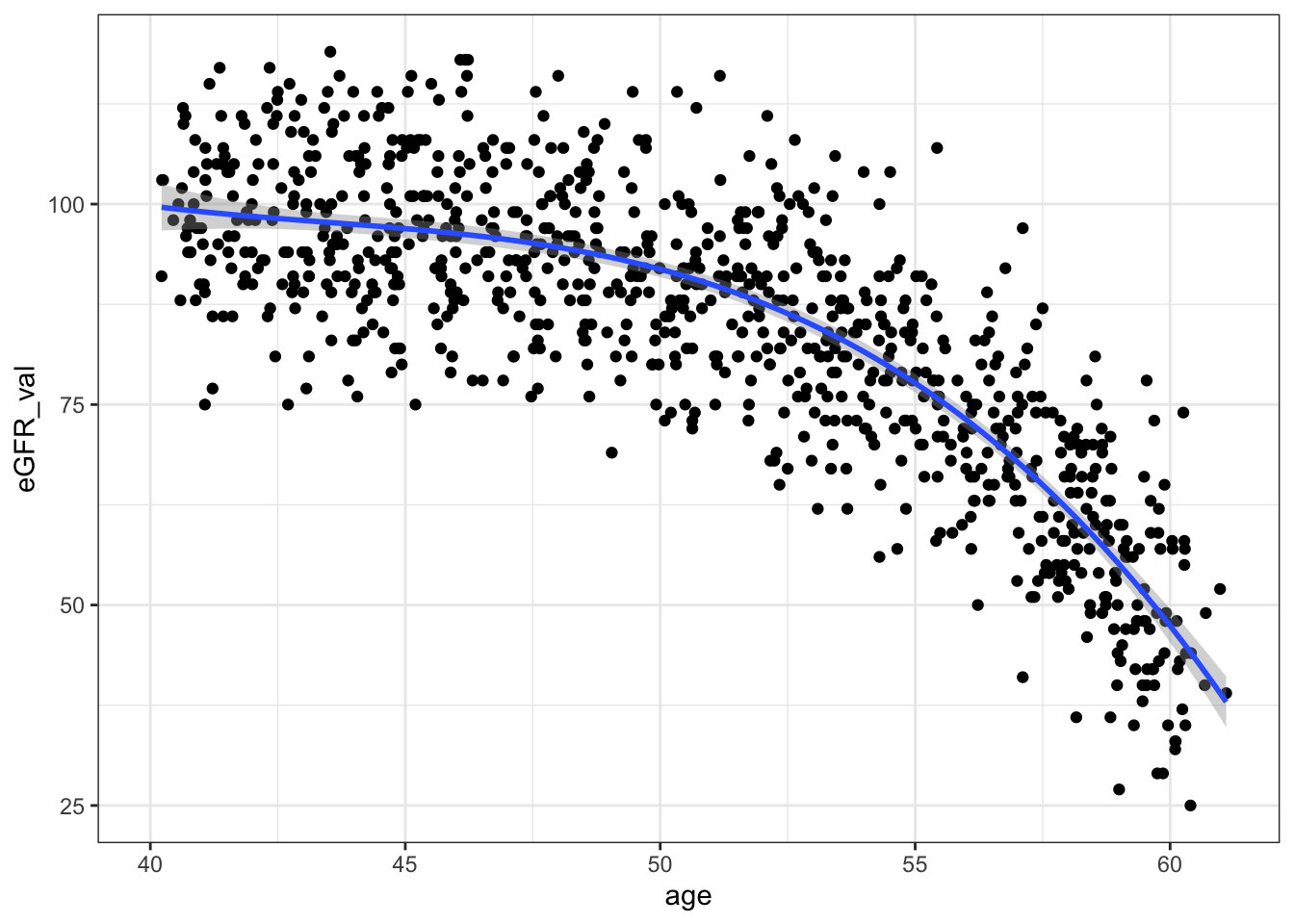
Or save the cleaned dataset for later use
saveRDS(pop, "cleaned_data.rds")Making it easy to load the dataset in at a later time without having to repeat the whole pipeline:
pop <- readRDS("cleaned_data.rds")